Deep dive
Adobe Mix Modeler is a unified, AI/ML powered measurement platform that combines multi-touch attribution (MTA) and marketing mix modeling (MMM) to deliver accurate, scalable, and future-proof marketing insights. This article presents a detailed breakdown of the methodology, design choices, and technical innovations behind Mix Modeler. And is based on this Summit 2025 session, which presents a detailed breakdown of the methodology, design choices, and technical innovations behind Mix Modeler.
As marketing complexity grows, traditional measurement approaches fall short. Fragmented data, evolving privacy constraints, and the need for both speed and rigor make it necessary to rethink how marketing performance is evaluated. Adobe’s response is Mix Modeler: an integrated system that uses machine learning to synthesize multiple data sources and modeling paradigms into a cohesive strategy.
This article explains the foundational components in more detail. These foundational components are:
- multi-touch attribution
- marketing mix modeling
- transfer learning (the intelligent exchange of outcomes between multi-touch attribution and marketing mix modeling)
Multi-touch attribution (MTA)
Overview
The multi-touch attribution (MTA) model that powers Mix Modeler is based on a discrete-time survival model trained on event-level data. Data includes searches, clicks, product views, add to carts, and checkouts. Using supervised learning, the model estimates the conditional probability of conversion at each step in the customer journey. The model considers both conversion and non-conversion customer journey paths to measure how different marketing touchpoints influence customer behavior over time. The non-conversion path is as important as the conversion path. The contrast between the two paths helps to understand whether a particular type of marketing touchpoint effectively drives conversion. For example, if one type of touchpoint appears as likely on a non-conversion path as on a conversion path, that touchpoint lacks impact on the conversion. This behavior is contrary to a touchpoint that appears often on a conversion path and not on a non-conversion path.
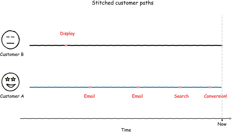
Key concepts
The key concepts behind multi-touch attribution are:
-
Interest modeling: Customer conversion is modeled as an accumulation of interest over time.
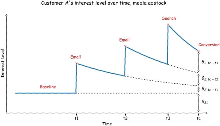
In this approach, a series of interest signals drive the likelihood of conversion, each influenced by
- prior media exposures,
- media adstock impact (a model of how responses to advertising build and decays in consumer markets), and
- other baseline factors.
These signals are represented as ϴBL + ϴE,tc-t1 + ϴE,tc-t2 and ϴS, tc-t3, where:
- ϴ: illustrates the model parameters (what is learned from the model).
- tc: the time of conversion.
- *tc-tx: the time between the exposure and the conversion, which is relevant for the model.
- BL: baseline.
- E: email.
- S: search.
In the modeling framework, the goal is to account explicitly for the time between each media exposure and the moment of conversion (tc-tx), recognizing that more recent interactions carry more weight than older ones.
-
Probability mapping: Conversion likelihood is derived from interest level using an S-shaped logistic function.
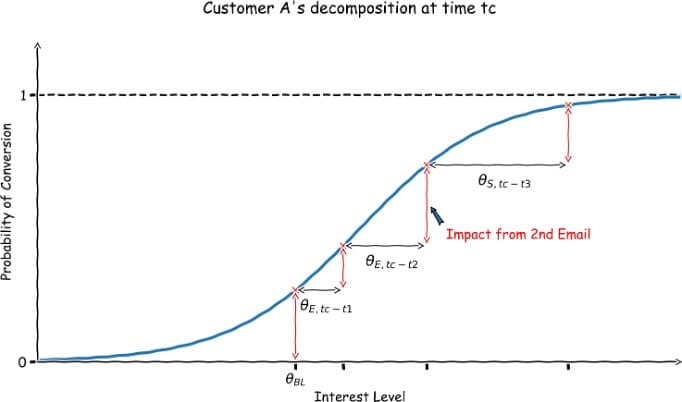
Through supervised machine learning that uses a discrete-time survival model, the above illustration visualizes customer A’s journey to conversion. The interest level is displayed on the X-axis and the probability of conversion on the Y-axis. This mapping shows that the second email (ϴE, tc-t2) exposure has the greatest impact on conversion. As indicated by a significant jump in the probability of conversion at the time of that step.
-
Diminishing returns: Additional touchpoints have less incremental impact as interest grows.
The S-shaped curve, from the illustration above, also shows that exposing the customer to additional touchpoints does have less incremental impact with growing interest levels.
-
Discrete-time survival model: Using a discrete-time survival model introduces more flexibility in the model, which allows the model to capture temporal nuances in customer behavior. The discrete-time survival model also relaxes some of the more restrictive assumptions required by continuous-time survival models.
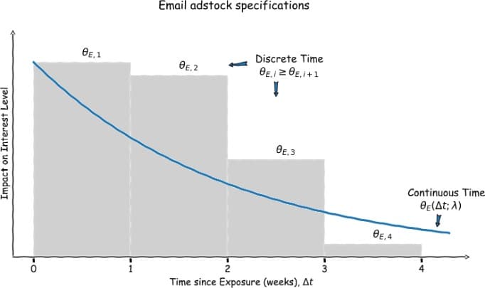
A continuous-time function models the impact of email adstock on the interest level, at any point in time since the time of exposure: ϴE(Δt;⋋)
A discrete-time function models the impact of email adstock on the interest level as discrete time windows using scalar parameters: ϴE,i ≥ 0E,i+1
Benefits
The multi-touch attribution approach selected for Mix Modeler has several key advantages.
- Account for both conversion and non-conversion paths, therefore ensuring a more accurate estimation of true media impact.
- Incorporate adstock and diminishing returns that model key real customer behavior and avoid oversimplified assumptions that are often found in rule-based models.
- Scale efficiently to large datasets due to the optimization for distributed computing and parallel processing.
- Support intuitive touchpoint attribution that allows for clear interpretation contrary to other methods such as Hidden Markov Models.
- Deliver strong performance and high predictive accuracy when compared against other classification algorithms.
Mix Modeler provides a marketer friendly interface to the insights resulting from multi-touch attribution.
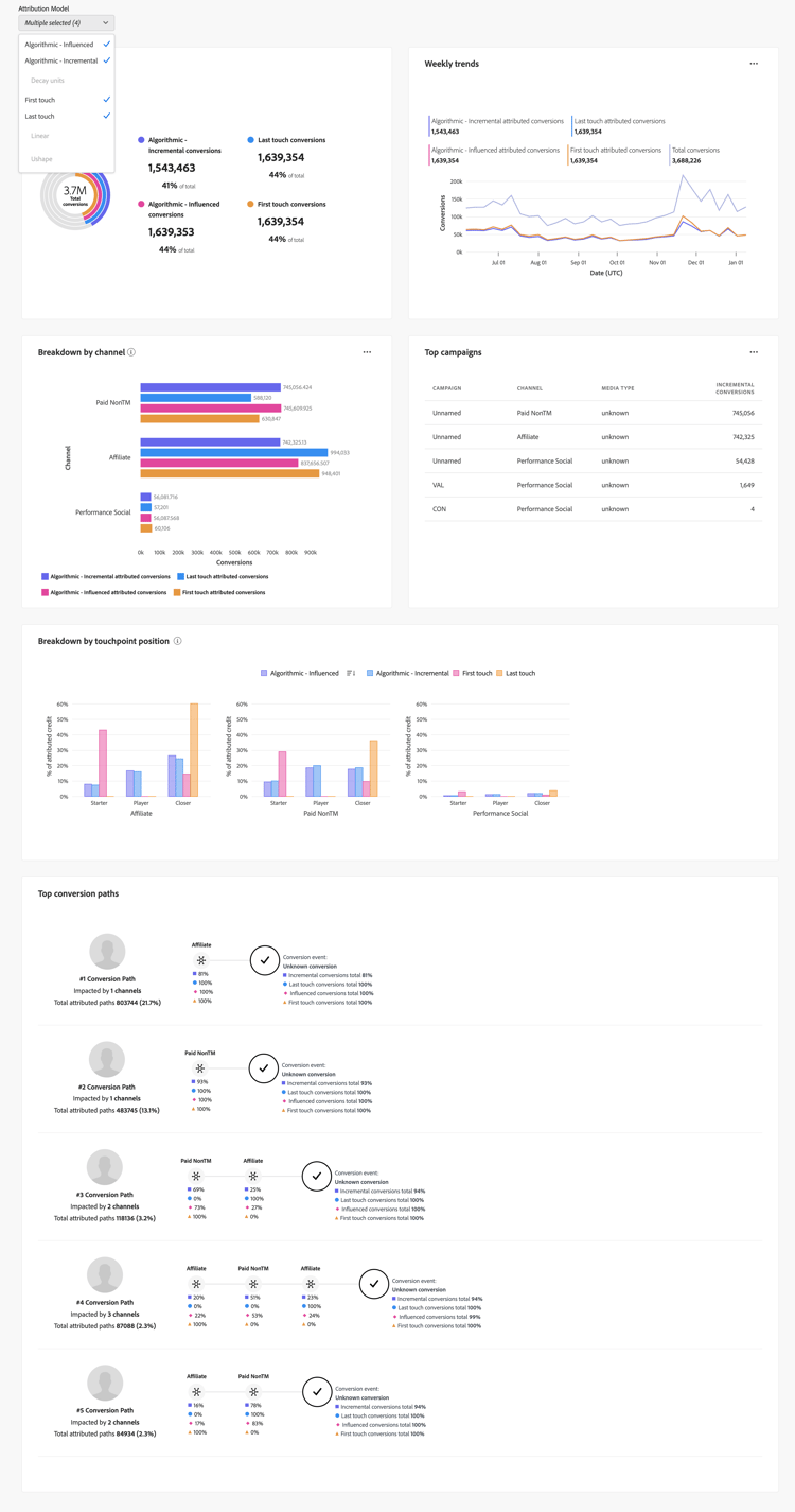
Although multi-touch attribution provides all these benefits, Mix Modeler does not rely in full on conversion insights from event-level data. Marketing mix modeling is another foundational component to take aggregate-level data into consideration.
Marketing Mix Modeling (MMM)
Marketing-mix modeling (MMM) is based on aggregate-level data and uses a multiplicative model structure, rather than an additive one, to reflect real-world marketing interactions.
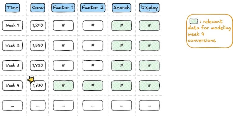
The illustration shows aggregate-level data in tabular format. Each row corresponds to a time period (usually a week, sometimes a day), and each column represents a variable. The table includes:
- the conversion column (the model’s outcome variable),
- media columns (for example: search, display), and
- factor columns (for example, seasonality, promotions) to capture internal or external influences outside of media spend that still impact media performance.
The model predicts week 4 conversions using the data highlighted in light green, including that week’s factors and historical inputs from media channels.
Key Concepts
The key concepts behind marketing mix modeling are:
-
Multiplicative model: Sales or conversions are the product of a baseline and media multipliers.
So, instead of using an additive model:
Weekly conversions = Baseline demand + Multiplier of Search + Multiplier of Display + …
use a multiplicative model:
Weekly conversions = Baseline demand x Multiplier of Search x Multiplier of Display x …Or in a formula: * Y = ⨍BL(Xfactors;θfactors) x ⨍S(XS;θS) x ⨍D(XD;θD)
For example:
-
Week actual conversions: 1730.
-
Week predicted conversions: 1787.5 = 1100 x 1.25 x 1.3, where:
- 1100: week 4 predicted baseline demand, a function for week 4 factor 1 and 2 data.
- 1.25: week 4 predicted search multiplier, a function from search data from week 1 through week 4.
- 1.3: week 4 predicted display multiplier, a function for display data from week 1 through week 4.
The anticipated difference between what the model predicts (1787.5) and the actual conversions (1730) is the residual, which is often small in size and not something to worry about.
-
-
Capture adstock and diminishing return: Adstock is captured using exponential decay and power functions.
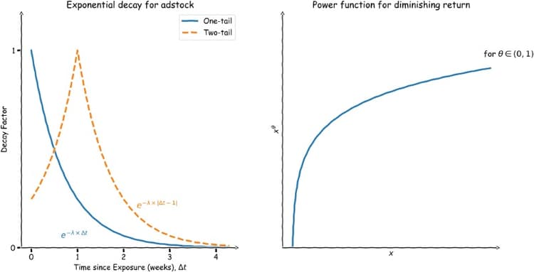
Exponential decay for adstock can be either one-tail or two-tail, depending on where the peak impact occurs after the media investment.
To take care of diminishing returns, the power function is applied: xθ for θ ∈ (0,1). This power function results in a concave shaped graph to capture the diminishing return. The diminishing return is then captured in the multiplier function within the MMM model.
Benefits
The benefits of the marketing mix modeling approach are based on the fact that the multiplicative model supports expected real-world marketing behaviors better. For example:
- Media synergy where media channels often work better together than in isolation.
- Time-varying impact where the same level of marketing investment can lead to different returns at different times due to external factors.
- Budget recommendations across time where expected market conditions or baseline fluctuations help to inform budget allocation over time.
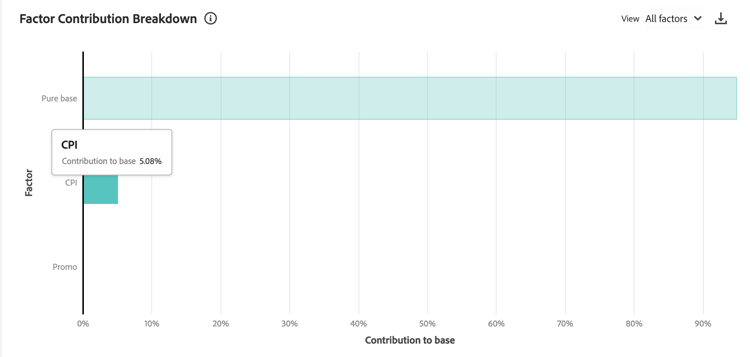
Mix Modeler provides a marketer friendly interface to the various insights resulting from marketing mix modeling. For example, a factor contribution breakdown to show the proportion of the base conversions that can be attributed to various factors included in the model.
Example
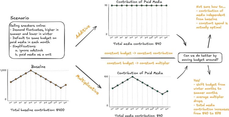
This simplified example illustrates how a multiplicative modeling approach for a fictitious sneakers online store allows for better budget allocation than the additive model.
Assumptions
-
Sneaker demand is higher in summer and lower in winter, as illustrated by Total baseline contributions.
-
The default strategy for marketing planning is to spend a fixed amount of marketing budget ($840) across the whole year, where each month gets the same budget.
-
Adstock is ignored and paid media is treated as a unit. These assumptions are independent of the chosen model and do not influence the comparison.
-
A constant budget in the additive model means a constant contribution across each month, which is reflected for the additive model on the top graph in the middle column.
-
In the multiplicative model, a constant budget means constant multipliers each month. To provide a time-varying impact for the same monthly spend, the multiplier works with the baseline demand. That multiplier effect is shown on the bottom graph in the middle column.
Move budgets
Is there any capacity to move away from a fixed budget, shifting the budget around, but keep the total budget to $840?
- In the additive model, there is no incentive from a modeling perspective to make a change as there is no interaction with the baseline. Having a flat spend is optimal. If you move $1 from November to May, the gain in May is smaller than the drop in November due to diminishing returns.
- In a multiplicative model, there is room to shift around. Based on the base line, you can shift budgets from winter months to summer months. The gain in the summer month is more than the loss in the winter month due to the multiplication effect. The extent of the shift and where to shift to is covered in the budget optimization algorithms used in marketing mix modeling.
Transfer learning
Next to multi-touch attribution and marketing mix modeling, experimentation is another important pillar in how to solve marketing measurement problems. Even though experimentation is not implemented within the framework of Mix Modeler, you can use experimentation, like turning off marketing in certain markets, to understand the causal impact of marketing on sales.
Adobe recommends and employs transfer learning to blend insights from multi-touch attribution, marketing mix modeling, experimentation, and other prior knowledge sources. This blending can be described as a layered approach. Each layer has gaps to illustrate the limitations in the production of a cohesive model. But if you stack the layers in the right way, you can compensate for the gaps in the combined model.
Apply this analogy when you use the combination of multi-touch attribution, marketing mix modeling, experimentation and prior knowledge sources. Blend these components in such a way that the combination suffers the least from flaws in each of the components.
In essence, transfer learning is numerical optimization algorithms at work. As part of model training, a loss function (to quantify the difference between a model’s predicted output and the actual (ground truth) value) is set up. And a goodness of fit metric (to evaluate how well a model’s predictions align with observed data) is determined. Transfer learning then solves the numerical optimization to get thetas (model parameters). If there’s one or more sources of information, that original optimization objective function is augmented with another term. That term measures the distance between what you supplied as prior knowledge and what the model produces to compare against.
Bi-directional transfer learning
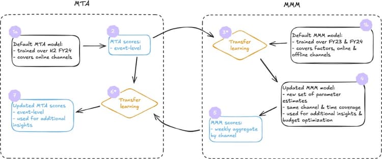
When you have both event-level data and aggregate-level data, bi-directional transfer learning involves the following workflow.
Consider the following:
- MTA is limited with respect to channel coverage (only event-level data from web and mobile data for example) but is advantageous due to the vast amount of data. The key aspect of MTA is relative performance.
- MMM understands the more holistic picture with factors, online, and offline channels.
- The transfer learning from MTA to MMM updates the MMM model. The transfer learning results influence the parameters that drive the multiplicative model. The transfer learning from MMM to MTA updates the MTA scores. There is no need to influence the MTA model as the initial scores are already statistically sufficient.
Prior knowledge
So beyond MTA, MMM, and experimentation, there are many other different sources of prior knowledge you can optionally leverage for marketing measurement planning. Different companies have different sources of prior knowledge. Examples include spend share, previous in-house models, or industry experience.
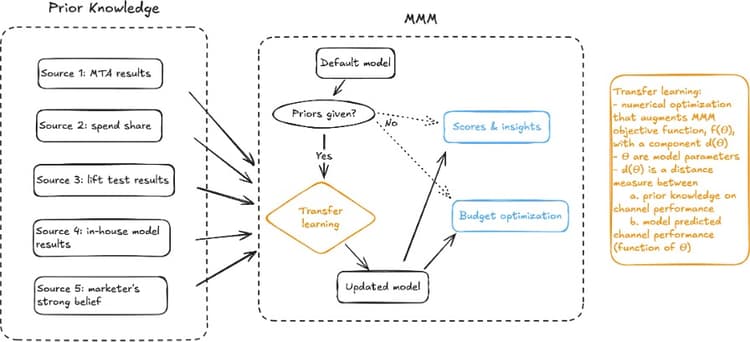
The model building process can leverage all these sources of information through the same transfer learning process. These prior knowledge sources are optional. You don’t need to have prior knowledge sources for marketing mix modeling to work. If you don’t have any prior knowledge, the default model is used to generate score insights and then budget optimization. If you do have prior knowledge input, you can use transfer learning to update the MMM model.
Budget optimization
Budget optimization is based on the multiplicative MMM model explained earlier,
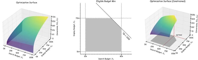
In a simple example, there are two channels: search and display. And you do have a total budget. The aim is to split the budget between the two channels to maximize conversion. Numerical optimization is used to find the optimal budget mix that maximizes the conversion under the total budget constraint. For example, imagine your total budget constraint is $130K.
The budget optimization formula is: Max ⨍(XS, XD) = ⨍BL(Xfactors) x ⨍S(XS) x ⨍D(XD), where XS and XD are parameters and Xfactors is forecasted.
Channel level constraints
Imagine you have additional channel level constraints:
- $10K - $80K for search.
- $5K - $70K for display.
- $130K in total.
As a result, the eligible budget mix causes the optimization surface to be constrained. The numerical optimization algorithm then helps to determine the optimal budget allocation.
Across multiple conversions
On top of channel level constraints, plan for optimal budget allocation across multiple conversions.
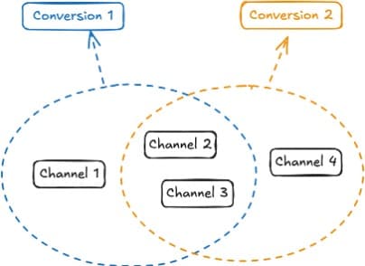
To accommodate optimal budget allocation across conversions, a weighted average of the above function for each of the conversions is used. The formula becomes ⨍new(X) = w1f1(X) + w2f2(X)
Examples of budget optimization across multiple conversions are:
- You want to maximize the total revenue from online sales and in-store sales conversions.
- You want to optimize for long term success using both brand awareness KPI and sales conversions.
In the second example, units of the two conversions are not similar (brand awareness KPI versus conversions) but that does not matter. Conversions or models do not have to refer to the same channels and can also overlap. Numerical optimization finds the best solution to the problem within the given constraints.
Summary
Adobe Mix Modeler is more than a measurement tool; Mix Modeler is a decision-support engine and its strengths are:
- The ability to model real-world complexity with statistical rigor
- A unified integration of diverse data and modeling paradigms
- A future-proof architecture that adapts to data deprecation trends
The combination of interpretability with performance has made Mix Modeler central to Adobe’s data-driven marketing transformation. Mix Modeler empowers marketing teams to make faster, smarter, and more aligned investment decisions.